Jari Kyngäs, Specialist Researcher, Business Intelligence Centers, SAMK
Kyngäs holds a PhD in computer science and is an expert in statistics and optimization.
Kimmo Nurmi, 0000-0001-8278-9874, Research Director, SAMK
Nurmi is an adjunct professor of computational intelligence and an expert in algorithms and optimization.
Keywords: Logistic regression, Odds ratio, Cross-tabulation, Classification, Prediction
Abstract
Logistic regression is a classification algorithm mostly used to predict a binary outcome based on independent variables. Put simply, we have explanatory factors whose values we use to determine whether the outcome of the event under consideration is more likely to be true or false. The method seeks to answer the question, "How can explanatory factors be used to predict whether an event will occur or not?" As in regression analysis in general, logistic regression seeks a mathematical connection between known inputs and known outcomes. The method is currently considered to be part of machine learning (or, more broadly, artificial intelligence), because the coefficients of the regression equation are calculated iteratively. The goal of this article is to increase understanding of how cross-tabulation, chi-square test, and logistic regression are used correctly, and how their incorrect use can be avoided. We present three serious pitfalls when using logistic regression: 1) using risk as a synonym for probability, 2) interpreting the individual coefficients of the explanatory factors provided by the model separately, and 3) an explanatory factor included in the logistic regression model is included in the final model even though it is not statistically significant in the model. We examine these pitfalls by looking at both sample data and statistical analyses from a study that received media attention.
1. Brief Introduction to Logistic Regression
Logistic regression is a classification algorithm used to predict a binary outcome based on independent variables. Put simply, we have explanatory factors whose values we use to determine whether the outcome of the event in question is more likely to be true or false. In other words, we want to know whether something will happen or not. Examples include whether a student will graduate or not, whether a team will win the championship or not, whether a person can be granted a credit card or not, whether an insurance claim is fraudulent or not, or whether an email is spam or not.
This article does not examine the mathematical foundations of logistic regression. A good article for this purpose includes (Osborne, 2014). As in regression analysis in general, logistic regression seeks a mathematical connection between known inputs and known outcomes. The method is currently considered to be part of machine learning (or, more broadly, artificial intelligence), because the coefficients of the regression equation are calculated iteratively. If the equation successfully models the connection between inputs and outputs, it can also be used to predict the correct output for new inputs (Logistic Regression, 2025).
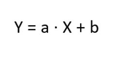
The reader should understand how logistic regression differs from the familiar linear regression. In linear regression, the answer is sought to the question "How can the values of X be used to predict the value of Y?". The value of Y is a real number. Mathematically expressed, formula (1) uses the least squares method (Rao and Toutenburg, 2008) to find the best values for the coefficient a, and the constant b. These coefficients are used to adjust the starting point and slope of the line shown in the example in Figure 1a). The figure shows that the need for insulin increases as weight increases.
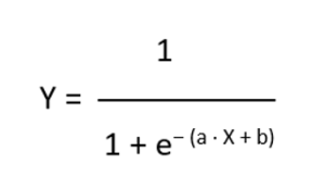
In logistic regression, the answer is sought to the question "How can X be used to predict whether Y is true or false?". The value of Y is binary, meaning it can only have two possible values, such as true/false or yes/no. Mathematically expressed, the maximum likelihood method (MLE) (Eliason, 1993) is used in formula (2) to find the best values for the coefficient a and the constant b. These coefficients are used to adjust the horizontal position of the line shown in the example in Figure 1b) and the steepness of the S-shape. The figure shows that the probability of diabetes increases with weight gain.

Logistic regression (almost) invariably involves several explanatory factors, in which case the parameter of the exponential function in formula (2) is presented in the form of a weighted sum.

In this case, the coefficient values are also optimized using the MLE method. The use of multiple explanatory factors in the model is only possible if the following necessary conditions are met:
- Only factors that have an explanatory effect can be included in the model.
- The explanatory factors are not mutually correlated.
- Each explanatory factor is a reasonable part of the model.
The basic information on logistic regression presented above is sufficient to begin examining serious pitfalls of its use. Problems associated with the use of logistic regression have been examined before (see, e.g. Bland and Altman, 2020; Knol et al., 2012; Persoskie and Ferrie, 2017), but to the best of our knowledge, not as concretely as in this article.
The goal of this article is to increase understanding of how cross-tabulation, chi-square test, and logistic regression are used correctly, and how their incorrect use can be avoided. We present three serious pitfalls when using logistic regression. In Chapter 2, we present the data used as an example, perform cross-tabulations, and examine the concepts of probabilities and risks. In Chapter 3, we examine whether statistical evidence can be found for the conclusions of the previous chapter using the chi-square test. In Chapter 4, we examine the findings of Chapters 2 and 3 using logistic regression. Finally, in the appendix, we describe how the study that received media attention made the mistakes described in this article in the use of logistic regression.
2. Sample Data, Cross-Tabulation, Probabilities and Odds
As an example, we consider data (Akin menetelmäblogi, 2014) that contains one multi-valued integer variable and two (binary) variables as explanatory factors, which can therefore only take two different values. This setup allows us to interpret the interactions between multiple variables. The explanatory variables in the data are:
Gender 0 = male, 1 = female
Marital status 0 = single, 1 = married
Income 0 - 75 000 (with an accuracy of 1000).
The event under consideration and prediction is "Based on the values of these three variables, how can we predict whether the person in question will buy the product or not?" We have 673 observations available for prediction, where buying is described by the variable:
Buying decision 0 = has not bought the product, 1 = has bought the product.
Before the current era of data analytics and artificial intelligence, cross-tabulation was by far the most popular method of analysis. Cross-tabulation is mainly used when the aim is to examine the effect of categorical and ordinal variables on each other. It should be noted that a good rule of thumb for cross-tabulation is that a maximum of 20% of the cells in the table should have fewer than five observations, and each cell should have at least one observation (Cochran, 1954). Correlation is often discussed in connection with cross-tabulation. It should be noted that correlation cannot be calculated between binary variables.
Let us begin our examination of the data by looking at the number of buyers and non-buyers broken down by gender and marital status (see Table 1).
Table 1: Number of buyers and non-buyers by gender and marital status.

These numbers can be us ed to calculate the probability of a person buying a product when we know their gender and marital status (see Table 2). For example, the probability of a person buying a product if they are male:

Table 2: Probabilities and risks of buying and not buying by gender and marital status.

Probabilities are easy to understand, and it is easy to make understandable relative comparisons between them. We use the term PR (probability ratio) for comparison. For example, a woman is 1.401 times more likely to buy a product than a man:

Next, we will take our first step toward pitfalls of logistic regression. In addition to probability, Table 1 can be used to calculate the so-called risk of a person buying a product when we know their gender and marital status (see Table 2). The term "bet" or "odds" is also used to refer to risk. Risk is calculated by comparing the probability of an event occurring to the probability of it not occurring. For example, the risk of a person buying a product if they are male:

Risk is more difficult to understand than probability. Risk is not usually used on its own, but rather as a relative comparison betw een two risks. In this case, we talk about odds ratio (OR) (Osborne, 2014) or betting ratio. Under no circumstances should the term risk ratio be used, as it is i n fact a ratio of probabilities as in formula (5). For example, the risk of a woman buying a product is 1.506 times that of a man (see Table 2):

The above does not mean that women are 1.506 times more likely to buy the product than men. It is 1.401 times more likely, as stated earlier. The odds ratio, i.e., the ratio between risks, is difficult to understand, as is risk itself. According to Table 2, married people are about 4.5 times more likely to buy than unmarried people. Furthermore, according to the table, the risk for married people to buy the product is about 6.5 times higher than for unmarried people. This difference certainly seems intuitively challenging, but fortunately, the correct use of logistic regression does not require an understanding of this difference.
Our topic is serious pitfalls of logistic regression, but at this point it is worth mentioning that, unfortunately, the odds ratio OR is too often used in relation to probabilities instead of PR, because OR is greater than PR (when OR is greater than one, see, e.g. (di Lorenzo et al., 2014). Thus, using it makes the result look better. This is based on the fact that the reader of statistical analysis does not understand the difference between, for example, the terms "4.5 times" (higher probability) and "6.5 times" (higher risk) in the previous wordings.
The odds ratio (OR) can be used in situations where data collection is challenging (e.g., expensive or laborious). In such cases, the researcher may find themselves in a situation where it is necessary to collect data on all observations related to the phenomenon under study, but other observations must be left out of the study. This leads to a situation where there are clearly more observations of the phenomenon under study than others in the data, i.e., the data set becomes distorted. This problem does not arise if the phenomenon under study is rare, because in that case the odds ratio gives an almost identical result to the probability ratio (PR). However, it should be understood that in practice no statistical method can be used on such distorted data.
Let's return to Table 2, from which we can visually conclude the following:
a. Gender has a minor influence on buying decisions.
b. Marital status has a major influence on buying decisions.
In the next chapter, we will examine whether there is statistical evidence to support these conclusions. Before that, let us take a look at income. We will classify income into low, medium, and high as follows:
Low < 50 000
Medium 50 000 - 74 000
High > 74 000.
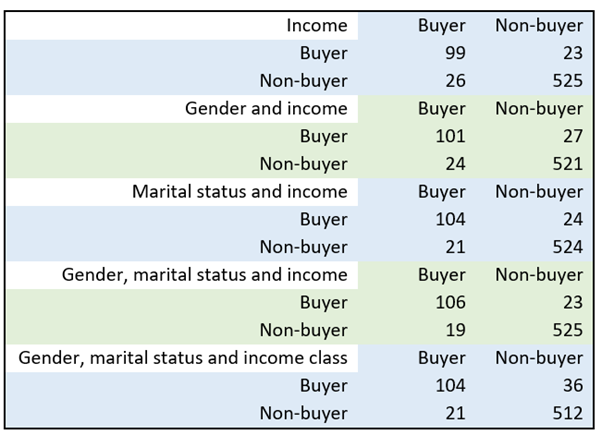
According to Table 3, people with medium incomes are about 20 times more likely to buy the product than those with low incomes, and those with high incomes about 40 times more likely. The risk of buying for people with low incomes is 11 / 481 = 0.023 and for those with high incomes 70 / 10 = 7. Since low income serves as the reference category for comparison, the odds ratio between these risks is 7 / 0.023, or approximately 306. Thus, the odds ratio explodes when one risk is small and the other is large. Similarly, the odds ratio between low income and middle income is approximately 34.
Table 3: Number of buyers and non-buyers broken down by income group.

3. Chi-square Test
Cross-tabulations must be subjected to an independence test to examine whether the variations in the values of the variables are statistically significant. The most commonly used test is Pearson's χ² test (chi-square test), which is based on a comparison of observed and expected values (Diez, Barr and Cetinkaya-Rundel, 2019).
We use the χ2 test to examine three dependencies:
- The effect of gender on buying decisions.
- The effect of marital status on buying decisions.
- The effect of gender and marital status on buying decisions.
Table 4: Effect of gender or marital status on buying decisions according to the χ2 test.

Table 4 shows the results when the χ2 test is used to examine the effect of gender or marital status on buying decisions. The expected value indicates the number that should be in the cell if the variables did not differ from each other, i.e., if they were independent of each other. The absolute value of the standardized residual reported by the test should be greater than 2, preferably greater than 3, in order to say that the observed and expected values differ from each other, i.e., in this case, there would be differences in buying behavior.
According to the test, the effect of gender on buying decisions is statistically significant with a p-value of 0.05. It should be noted that if even one woman's buying decision in the data set had been a non-buying decision, the test would no longer have been significant. In that case, the conclusion would have been that gender has no effect on buying decisions.
Statistical significancy has been largely criticized for a long time but especially for the last ten years (see e.g. Reinhart, 2015; Greenland et al., 2016). We are not going into detail here but most of the criticism has been directed to whether or not decisions can be made strictly based on p-values. The discussion in previous paragraph is a good example of this. We understand the criticism and we hope the appendix helps in understanding why we focus on p-values.
The effect of marital status on buying decisions is statistically significant, with a p-value of less than 0.01. This can be seen in Table 4, where the actual observation values deviate significantly from the expected observation values. In addition, the absolute value of the residual is clearly above 3. The conclusion is that married people buy significantly more of the product than unmarried people. Table 4 shows that 88 married people bought the product, but only 44 would have bought the product if married people behaved like unmarried people.
Finally, let us examine the effect of gender and marital status on buying decisions (see Table 5). According to the test, their effect (i.e., the four different groups) on buying decisions is statistically significant, with a p-value of less than 0.01. Married women are more likely to buy the product than others, and married men are also more likely to buy it than unmarried women and men. Married people are therefore more likely to buy the product than unmarried people. Gender does not seem to have a significant effect.
Table 5: The effect of gender and marital status on buying decisions according to the χ2 test.

Table 6: Comparison of buying probabilities.

Let us calculate the relative comparisons of buying probabilities according to formula (5) from Table 5 to Table 6. The first row tells us that married women are about four times more likely to buy the product than unmarried women. The first two rows show, as previously stated, that married people are more likely to buy the product than unmarried people (regardless of gender). Marital status therefore has a significant impact on purchasing behavior. Again, gender does not appear to have a significant impact. Please note that we are not presenting risks or odds ratios at this point.
In the next chapter, we will examine the findings of Chapters 2 and 3 using logistic regression.
4. Logistic Regression
Chapter 1 provided a brief introduction to logistic regression. In this chapter, we apply the method to all eight variations of the three explanatory variables in the data set. At this point, it should be noted that the necessary conditions described in Chapter 1 are met:
- Only factors that have an explanatory effect can be included in the model.
- The explanatory factors are not mutually correlated.
- Each explanatory factor is a reasonable part of the model.
From the perspective of this article, there is no need to go into greater depth on models formed using logistic regression. Statistical software produces the odds ratio (OR) values shown in Table 7 when using logistic regression.
Table 7: Probabilities and risks of buying and not buying by gender and marital status.

The table shows that when logistic regression is used with a single explanatory variable (gender or marital status), the OR values obtained are exactly the same as those calculated earlier (see Table 2). Let us examine gender in more detail. The statistical software produces values of a = 0.409 and b = -1.717 for the coefficients in formula (2). Since gender can only have values of 0 and 1, we obtain the values in Table 8 when substituted into formula (2).
Table 8: Result of the logistic regression equation when we examine gender.

The values 0.152 (male) and 0.213 (female) in the table are exactly the same as those we calculated earlier (see Table 2). Cross-tabulation and logistic regression therefore give us the same answers in the case of a single explanatory variable. At this point, however, it is important to note that logistic regression is not intended to be used in the case of a single binary explanatory variable.
The use of logistic regression requires at least one explanatory factor in the data set that is a multivalued real or integer variable. In our example, this is income. Let us look again at Table 7. We can see that the odds ratio increases for gender and decreases for marital status to approximately 4. This is due to the combined effect of all three explanatory factors on the weighted sum in formula (3).
This brings us to the most important point of this article and the most serious pitfall of logistic regression: the individual coefficients of the explanatory factors in logistic regression cannot and must never be interpreted separately! This interpretation is only possible when there is exactly one explanatory factor. As already stated above, in this case it is advisable to use cross-tabulation in addition to logistic regression. Let us state once again that logistic regression describes the combined effect of all explanatory factors, so they can only be examined together, not separately.
Based on the numbers in row four of Table 7, we cannot say that the risk for women is 1.37 times higher than for men. The first row of the table shows that it is 1.5 times higher.
Instead, we could say that the risk for married women to buy the product is about 1.5 times higher than for married men when marital status is also considered. However, we cannot say this either, because the results of the logistic regression statistical model show that gender is not statistically significant. This means that this model might not be suitable. Note that earlier cross-tabulation showed that gender has no significant effect on buying decisions.
Let us return to the previous observation, namely that the odds ratio increases for gender and decreases for marital status to approximately 4. Interpreting only the odds ratio, we could say the risk for women to buy the product is four times higher than for men. It could also be said the risk for married people to buy the product is four times higher than for unmarried people. Based on the last three rows of the table, it appears that gender and marital status have an equal impact on the buying decision. We have already stated several times that this is not the case. Marital status should have a significant effect on the buying decision, but gender should not. Why does the logistic regression according to Table 7 suggest otherwise?
Based on the last three rows of the table, we could interpret that gender and marital status have an equal impact on purchasing decisions when income is also considered. That is because the table shows that the risk caused by gender and marital status is the same for both, i.e., fourfold. Or, more precisely, the risk for both women and single people to buy the product is four times higher when income is also considered. In this data set, logistic regression clearly overemphasizes the effect of gender on buying decisions. The reason for this is the combined effect of the explanatory factors on the regression equation, as emphasized several times earlier.
Finally, let us examine the explanatory factors in the last row of Table 7, namely gender, marital status, and income classes, and the logistic regression model formed for them. The statistical software produces the coefficients of formula (3) presented in Table 9. Using these coefficients, formula (2) gives a buying probability of 0.959 for a married woman with a high income and a buying probability of 0.155 for an unmarried man with a medium income.
Table 9: Results of the logistic regression equation when we examine gender, marital status, and income classes.

5. Predictive Ability of Logistic Regression
In this chapter, we examine the predictive power of logistic regression. For this purpose, the method produces a confusion matrix. The matrix shows how many times actual observations are misclassified when values produced by the regression equation generated by the method are used instead. The confusion matrix divides the data classified by explanatory factors into four categories according to the event being examined: correctly positively (true) predicted, correctly negatively (false) predicted, incorrectly positively predicted, and incorrectly negatively predicted. Statistical software produces the confusion matrix shown in Table 10 when income is included as an explanatory factor. The number 26 in the second row means that of the 125 people who actually bought the product, the regression equation incorrectly placed 26 in the non-buyer category.
Table 10: Confusion matrix when income is included as an explanatory factor.
The differences in the table seem minor. When calculating the confusion matrix, statistical software generates the following four key figures (see, e.g. Diez, Barr and Cetinkaya-Rundel, 2019) to help interpretation:
Accuracy Percentage of correctly predicted cases (overall predictive ability)
Precision Percentage of correctly predicted positive cases out of all predicted positive cases (accuracy of positive predictions)
Recall (Sensitivity) Percentage of correctly predicted positive cases out of all actual positive cases (accuracy of actual positive cases)
F1 Harmonic mean of precision and recall.
A high F1 score indicates that the model is capable of accurately predicting positive cases and minimizing false positives and false negatives.
Table 11 shows the key figures (in percentages) produced by calculating the confusion matrix. Based on these key figures, we can make the following observations. When gender is used as a second explanatory variable in addition to income (second row), the predictive power of the model deteriorates. The model is only better in terms of the Precision indicator (80.80%), i.e., its ability to predict buyers. When marital status is added as a second explanatory variable in addition to income (third row), the model's predictive power improves in all respects and clearly in its ability to predict buyers (83.20%) while simultaneously minimizing false positives and false negatives (82.21%). When gender is added (fourth row), the difference is mostly marginal. When income classes are used instead of income, the accuracy of the prediction decreases because we lose known information through classification. As a rule of thumb, it can be said that the key figures should be above 80% for the model to be considered good. In conclusion, we can once again state that marital status has a significant impact on purchasing decisions, but gender does not.
Table 11: Key figures produced by calculating the confusion matrix (as percentages).

6. Conclusions
Logistic regression is a classification algorithm used to predict a binary outcome based on independent variables. The method seeks to answer the question, "How can explanatory factors be used to predict whether an event will occur or not?"
The use of multiple explanatory factors in the model is only possible if the following necessary conditions are met:
- Only factors that have an explanatory effect can be included in the model.
- The explanatory factors are not mutually correlated.
- Each explanatory factor is a reasonable part of the model.
The first pitfall of logistic regression discussed in this article is using risk as a synonym for probability (1). Risk is not usually used on its own, but rather as a relative comparison between two risks. This so-called odds ratio is also unfortunately often used as a synonym for probability relations. Even if the researcher understands this, the reader of the study will most likely not. It would therefore be advisable to pay less attention to interpretations related to both risk and odds ratio.
The second and most serious pitfall associated with logistic regression is interpreting the individual coefficients of the explanatory factors provided by the model separately (2). Logistic regression reveals the combined effect of all explanatory factors, so they can only be examined together, not separately. Logistic regression should be used for its intended purpose, i.e., classification. No conclusions should be drawn from individual coefficients, as all explanatory variables influence each other. If one explanatory variable is removed from the model, the coefficients change. If one explanatory variable is added to the model, the coefficients change. And these coefficients are used to calculate the risk mentioned earlier.
The third pitfall is that an explanatory factor included in the logistic regression model is included in the final model even though it is not statistically significant in the model (3). In this case, condition 1 above is not met. This means that this model cannot be used. The reason for this is that all explanatory factors in the model influence each other and, through this, the coefficients mentioned in the previous section.
We used an example to explain how to interpret the results produced by logistic regression and how to use them safely and correctly. However, we recommend that researchers use cross-tabulation and the χ2 test instead of, or at least in addition to, logistic regression.
The final conclusion of the analysis of the data used in the example is that the higher the income, the more likely a person is to buy the product. In addition, marital status has a significantly greater impact on buying decisions than gender.
Appendix
In this appendix, we examine a study (Savinainen et al. 2020) that uses logistic regression. The Finnish state-owned national media company YLE has published the results of the study (Kangas, 2020).
The study concludes that: "A higher body fat percentage and exposure to parental smoking in girls aged 6-8 years are independent predictors of prethelarche, i.e. preliminary breast development (secondary development of the mammary glands before puberty)." Table 12 shows the cross-tabulation of smoking and prethelarche, as well as the χ2 test.. According to the test p-value of 0.1429, smoking has no effect on prethelarche in girls. As the value is clearly above 0.05, it can be said that this data does not show that parental smoking affects prethelarche. However, the results of this χ2 test are not presented in the study. Instead, the results of logistic regression have been used and presented.
Table 12: Effect of smoking on prethelarche according to the χ2 test.
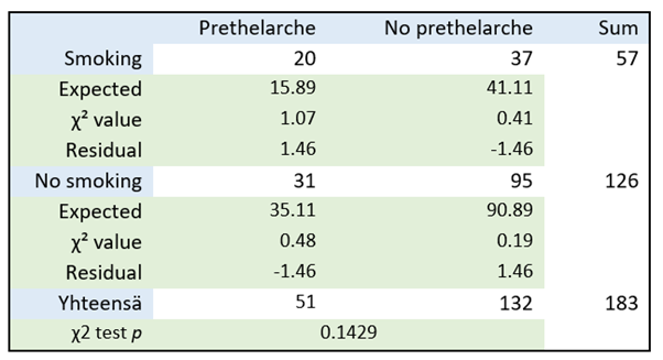
Table 13: Probabilities, risks, and their relationships.
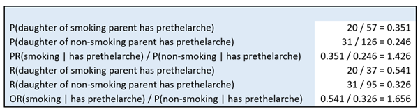
The probabilities and risks discussed in the main article, as well as their relationships, can be calculated from the table. According to the figures in Table 13, girls with smoking parents are approximately 1.43 times more likely to experience prethelarche than girls with non-smoking parents. Similarly, the risk of prethelarche in girls with smoking parents is approximately 1.66 times higher than in girls with non-smoking parents. As stated in the main article, it would be advisable to pay less attention to interpretations related to both risk and cross-ratios. It should be noted here that the main finding of the study (Savinainen et al. 2020) and the news report (Kangas, 2020) was that "parental smoking increased the likelihood of premature breast development by 2.6 times."
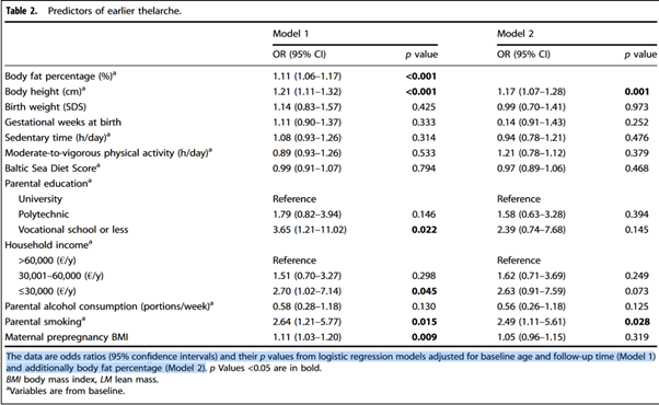
The study examined 14 possible explanatory factors, which are presented in Figure 2.
Let us remember that logistic regression may only be used if the following necessary conditions are met:
- Only factors that have an explanatory effect can be included in the model.
- The explanatory factors are not mutually correlated.
- Each explanatory factor is a reasonable part of the model.
The second and third points can be assumed to be true in this case. Two logistic regression models were calculated in the study. The results are presented in Figure 2. The first model includes 14 possible explanatory factors, and the second model includes 13. The table shows that, according to the first model, only six of the possible explanatory factors are significant (p < 0.05):
- Girl's body fat percentage (real number with one decimal places)
- Girl's height (real number with one decimal places)
- Parental education, if vocational or lower (ordinal scale, three categories, with university education as the reference category)
- Household income, if no more than 30,000 €/y (ordinal scale, three categories, with the highest income as the reference category)
- Parental smoking (binary)
- Maternal prepregnancy BMI (real number with one decimal places).
The study does not explain why the researchers decided to fit another model, from which they removed the girl's body fat percentage. It seems they thought that controlling for body fat percentage means it is a confounding factor which would reveal that some of the explanatory factors are bind to it. They concluded that after controlling for body fat percentage lower parental education and higher maternal prepregnancy BMI are explained with it. The conclusion was based on the observation that these two explanatory variables were not statistically significant after removing body fat percentage from the logistic regression. However, there were already a lot of statistically insignificant explanatory variables in the logistic regression, which they did not comment on at all. All of these non-significant explanatory variables do affect the outcome of the logistic regression.
They then fitted a new logistic regression model for the remaining 13 possible explanatory factors. The table shows that, according to the second model, only two of the possible explanatory factors are significant (p < 0.05):
- Girl's height (real number with one decimal places)
- Parental smoking (binary)
The study results state that "Girls who had a parent who smoked were 2.64 times more likely to have premature breast development than other girls." This coefficient is taken from the first model, where it is higher than the 2.49 in the second model. Let us return to the three serious pitfalls mentioned in the main article when using logistic regression:
- Risk is used as a synonym for probability.
- The individual coefficients of the explanatory factors provided by the model are interpreted separately.
- The final model includes possible explanatory factors included in the preliminary model, even if they are not statistically significant in the preliminary model.
The study has fallen into all three of these pitfalls:
- According to the wording of the main results of the study, "Girls who had a parent who smoked were 2.64 times more likely to experience premature breast development than other girls" or "Parental smoking increased the likelihood of premature breast development by 2.6 times." The risk has been incorrectly used as a synonym for probability.
- The single coefficient (2.64) given by the model for one explanatory factor (smoking) has been misinterpreted separately.
- The interpretations of both models (which are already incorrect in themselves) have been misinterpreted from preliminary models that included explanatory factors that were not statistically significant.
To understand these pitfalls, we refer to the content of Chapter 4 of the main article and, in particular, to the discussion related to row four of Table 7. In addition to the pitfalls mentioned in the study, there are other points that raise questions. Firstly, there are only 183 observations, so it is highly likely that only a few statistically significant explanatory factors will remain in the final model.
The strengths and limitations section of the study points out that there's not enough info on when the girls' breasts started growing, when their parents hit puberty, and how long they were exposed to smoking. It is therefore not known whether the girls were even exposed to smoking. The only information available is that at least one of the parents smoked, but there is no information on whether they smoked in the presence of their daughter.
An important finding was that the girl's exposure to parental smoking was a strong predictor of prethelarche even after body fat percentage had been controlled for, i.e., removed from the model. This finding was based on the fact that one statistically significant explanatory factor had been removed from the first model, but eight statistically insignificant explanatory factors had been left in.
In addition, the study concluded that lower parental education, lower household income, and higher maternal pre-pregnancy body mass index were also associated with earlier onset of pregnancy. However, the association between parental education and maternal prepregnancy BMI with the age of thelarche was largely explained by girls' body fat percentage, and the association with household income was partly explained by girls' body fat percentage.
Finally, we note that the study did not publish the logistic regression equation for the models created, and the goodness of the model in predicting the prethelarche was not reported.